Illustrations
This page contains all the figures and illustrations from The Geospatial Desktop
Click on an image to view a larger version and page through each image.
If you prefer, you can download a PDF (17Mb) containing all illustrations.
All images are Copyright © 2012, Gary Sherman
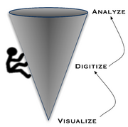
3.1 – GIS functions
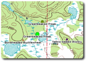
3.2 – Bird sightings: The bigger the dot, the more birds
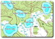
3.3 – A 200-foot buffer around the lakes
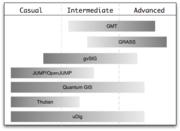
4.1 – Some OSGIS applications in relation to class of user
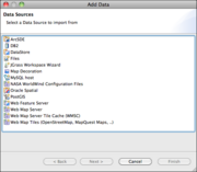
5.1 – uDig Data Sources Dialog
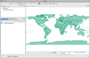
5.2 – uDig displaying world borders
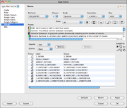
5.3 – Classifying countries by population
5.4 – Countries classified by population
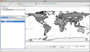
5.5 – Viewing attributes in uDig

5.6 – QGIS with sample data loaded
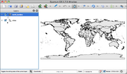
5.7 – QGIS vector layer properties
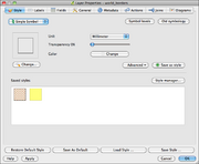
5.8 – Nicely rendered world_borders layer
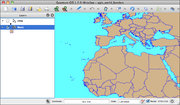
5.9 – QGIS continuous color renderer settings
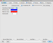
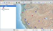
5.10 – QGIS continuous color renderer results
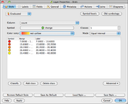
5.11 – QGIS graduated renderer settings
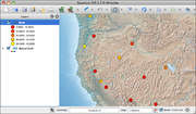
5.12 – QGIS graduated renderer results
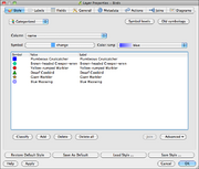
5.13 – Unique value renderer for birds
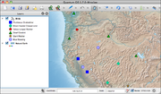
5.14 – Viewing birds by name
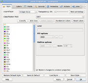
5.15 – QGIS unique renderer settings for a geologic map
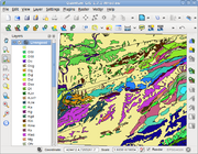
5.16 – QGIS unique renderer result
5.17 – QGIS Identify results
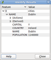
5.18 – Attribute table for the cities layer
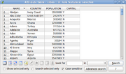
5.19 – Search Query Builder
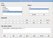
5.20 – Attribute action enabled in QGIS
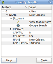
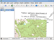
6.1 – Montana topographic map in QGIS
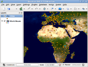
6.2 – NASA world mosaic viewed in QGIS
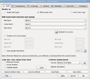
6.3 – QGIS raster properties dialog box
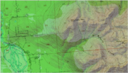
6.4 – Semitransparent digital elevation model draped over a DRG
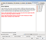
6.5 – QGIS raster pyramids dialog box
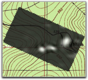
6.6 – Grid of silver values
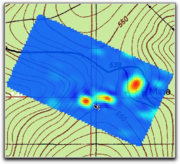
6.7 – Grid of silver values in pseudocolor
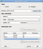
7.1 – Creating a new shapefile in QGIS
7.2 – QGIS with new layer ready to edit
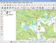
7.3 – Entering attributes for a feature
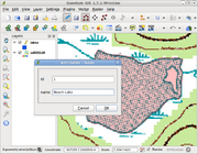
7.4 – Results of digitizing lakes in QGIS
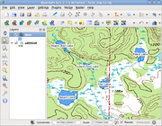
7.5 – Digitized Streams
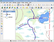
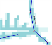
7.6 – Problems with the digitized streams
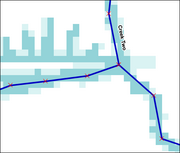
7.7 – Digitized streams with corrections
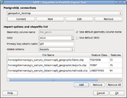
9.1 – Loading shapefiles into PostGIS using SPIT
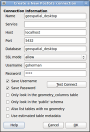
9.2 – Creating a new PostGIS connection in QGIS
9.3 – List of available PostGIS layers
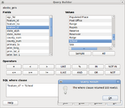
9.4 – PostGIS query builder in QGIS
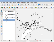
9.5 – PostGIS layers created with the query builder
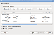
9.6 – PostGIS connect dialog box in uDig
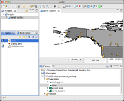
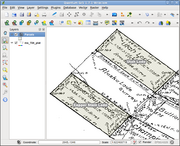
10.1 – Digitizing a plat
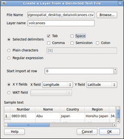
10.2 – The QGIS Delimited Text plugin
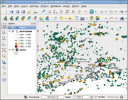
10.3 – Earthquakes rendered in QGIS by magnitude
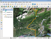
10.4 – GPS plugin in QGIS

10.5 – Track and waypoint loaded from GPS unit
10.6 – Uploading to the GPS

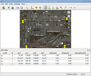
10.7 – Georeferencing an image with QGIS
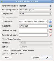
10.8 – Transformation Settings for Georeferencing an Image with QGIS
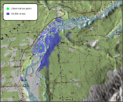
12.1 – Results of line-of-sight analysis in GRASS
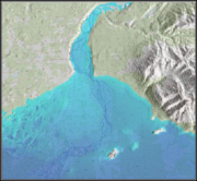
12.2 – Raising sea level by 100 meters
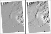
12.3 – Hillshade with no exaggeration (left) and 4X exaggeration (right)
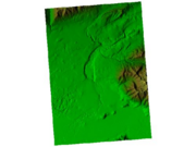
12.4 – Colored shaded relief map created with GRASS
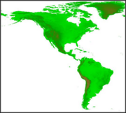
12.5 – Merged GTOPO30 DEM
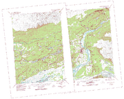
12.6 – Overlapping collars on DRGs
12.7 – Seamless display of clipped DRGs
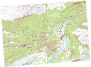
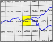
12.8 – Rivers and the quadrangle for clipping
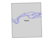
12.9 – Rivers clipped to a quadrangle boundary
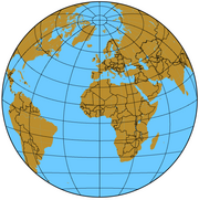
13.1 – Hemisphere view of Earth created with GMT
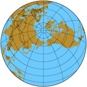
13.2 – Globe centered on 180/65
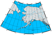
13.3 – Alaska coastline generated with GMT
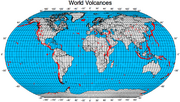
13.4 – Volcanoes plotted on a Robinson projection using GMT
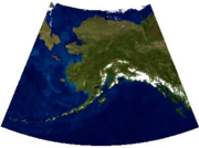
13.5 – Alaska derived from the world mosaic

13.6 – Alaska mosaic warped to Alaska Albers projection
13.7 – VRT raster over the parcel shapefile
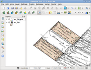
14.1 – The GRASS Plugin Toolbar

14.2 – Selecting a GRASS mapset in QGIS

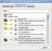
14.3 – The GRASS tools in QGIS
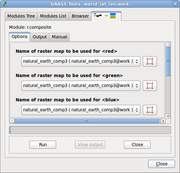
14.4 – The GRASS Toolbox Ready to Run r.composite
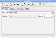
14.5 – GRASS edit tools in QGIS
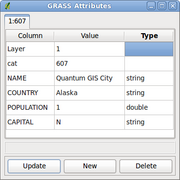
14.6 – Adding attributes to a GRASS feature
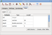
14.7 – Adding columns to the new GRASS map table
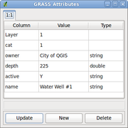
14.8 – Editing the attributes of an existing feature
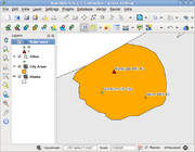
14.9 – Completed city map with water wells
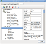
14.10 – GRASS browser in QGIS
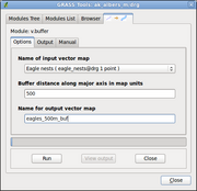
14.11 – Buffer module ready to buffer eagle nest locations
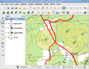
14.12 – Buffered eagle nests created with GRASS and QGIS
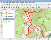
14.13 – Roads buffered using GRASS in QGIS
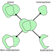
14.14 – Result of each type of vector overlay operation
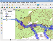
14.15 – Timber stands and stream buffers
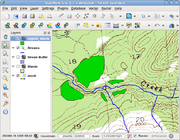
14.16 – Eligible logging areas after vector subtraction
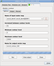
14.17 – Setting up to contour a DEM
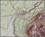
14.18 – Result of contouring the DEM
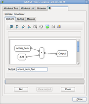
14.19 – Mapcalc model for converting DEM from meters to feet
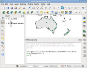
15.1 – Changing the window title with Python
15.2 – Installing the Plugin Builder

15.3 – Plugin Builder Ready to Generate the Zoom to Point Plugin

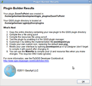
15.4 – Results of Generating the ZoomToPoint Plugin
15.5 – Plugin dialog box in Qt Designer
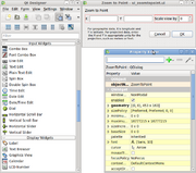
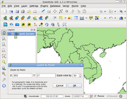
15.6 – ZoomToPoint plugin in use
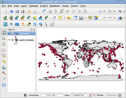
15.7 – Volcanoes shapefile created with Python script
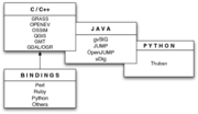
16.1 – Applications grouped by underlying programming language
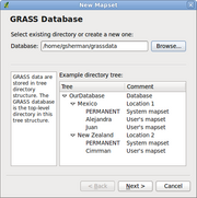
18.1 – GRASS database selection/creation dialog box
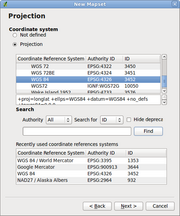
18.2 – Choosing the WGS 84 projection for the GRASS location
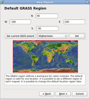
18.3 – Default region settings for a WGS 84 world location
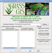
18.4 – GRASS start-up form
18.5 – GRASS location parameters
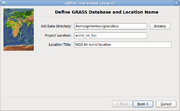
18.6 – GRASS location and mapset created and ready to use
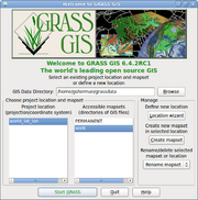
18.7 – World mosaic in GRASS
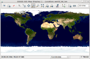
18.8 – GRASS thematic map showing world population
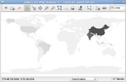
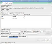
18.9 – Adding a Column to a GRASS Vector Map
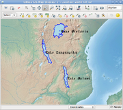
18.10 – Results of digitizing lakes in GRASS
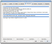
19.1 – Metadata for the world_borders layer
19.2 – QGIS Geospatial Bookmarks dialog box

19.3 – QGIS Plugin Manager
