
Creating an Annotated Map with GMT
For this example, we’ll create a map of Alaska and annotate it. If you looked at the Simple Globe example you’ll recall that the -R switch controls the extent of a GMT map. Alaska ranges from about 172 degrees east longitude to 130 degrees west. Using 360 degrees for the entire globe, this translates to a region extending from 172 degrees to 230 degrees. For the Alaska map we will use the Albers Equal Area Conic projection. Looking at the syntax for pscoast reveals that this requires the use of the -Jb switch. In this case, we use the lowercase “b” to indicate that we will specify the size of the map using a scale. First lets look at the command used to create the map:
pscoast -Jb-154/50/55/65/1:12000000 -R172/230/51/72 -B10g5/5g5 -W1p/0/0/0 \

-I1/2p/0/192/255 -I2/2p/0/192/255 -I3/1p/0/192/255 -I4/1p/0/192/255 \

-G220/220/220 -S0/192/255 -L210/54/54/1000 -P -N1/1p/0/0/0 -Dl >gmt_alaska_coast.eps
This looks like quite a complex command, but it’s really not too bad once you get past all the numbers and slashes.
Projection
First note we specified the projection using -Jb-154/50/55/65/1:12000000. Lets pick that apart a bit to see what’s happening. The Albers projection requires the longitude of the central meridian, the latitude of the origin, and the latitude of the two standard parallels. That’s what you see specified as -154/50/55/65. These are the standard values used for the Albers projection in Alaska. You can actually specify any values you want, but if there is a standard for the area you are mapping you should use it.
The remaining part of the -Jb switch is the size of the output. In this case we specified it as a scale of 1:12,000,000. This means that one unit on the map represents 12,000,000 units on the ground (in this case meters). If we just wanted output to fit on a page, we could specify -JB-154/50/55/65/6.0i to get a 6-inch wide image.
Map Extent
To set the map extent we use the -R switch. In this case we already determined that Alaska ranges from 172 to 230 degrees longitude and roughly 51 to 72 degrees north latitude. To create the map covering this area, we use -R172/230/51/72.
Grid Lines
In this example we not only want to draw grid lines, but also want to annotate them. This is done using -B10g5/5g5. This tells pscoast to draw grid lines 5 degrees apart for both latitude and longitude. The annotation is drawn at 10 degree intervals for longitude and 5 degree intervals for latitude. If you look at the documentation for pscoast you will see that the first number after the -B is the annotation interval followed by the grid line interval. This notation gives you a lot of flexibility in drawing and labeling gridlines.
Rivers
To make our map more interesting, we’ll add rivers to it. GMT comes with several levels of river detail which are specified with the -I switch. The levels we are using are:
- Permanent major rivers
- Additional major rivers
- Additional rivers
- Minor rivers
Notice the -I options we specified in the pscoast command. One is required for each river level we want to include on the map. The first two (major rivers) are drawn using a pen width of 2 (2p), while the third and fourth level are drawn with a width of 1 (1p). We use the same color (0/192/255) for each river. If we wanted to include the intermittent major rivers (fifth level) we would add -I5/1p/0/192/255 to the pscoast command.
Fill Colors
Next we specify the fill colors for the land and water areas using the -G and -S switches and add the RGB values to specify the color. For land we use a light gray with RGB values of 220/220/220. For the water 0/192/255 gives us a nice cyan color. Keep in mind that we could also use a pattern or shade for filling land and water areas.
Scale Bar
A scale bar can easily be added to the map using the -L switch. Scale bars can be simple or fancy. In this case we’ll just create a simple one and place it in an open area on the map. How do we know it’s open? Well part of the process is running pscoast and tweaking the options, then running it again until we get the look we want. To create the scale bar we need the latitude and longitude of the point where we want to place it. Since scale varies as we move further from the equator, we also specify the latitude at which we want the scale calculated. Lastly we indicate the length the scale bar should span. The default is kilometers but you can append m for miles or n for nautical miles. Putting it all together we have -L210/54/54/1000 which gives a 1,000 km scale bar calculated at 54 degrees north latitude and originating at 210 degrees longitude and 54 degrees latitude.
The Last Bits
The remainder of the command tells pscoast to use portrait mode (-P), draw country boundaries in black using a pen width of 1(-N1/1p/0/0/0), and use the low resolution data (-Dl). The low resolution data set is the default but we specified it here so you could see the syntax.
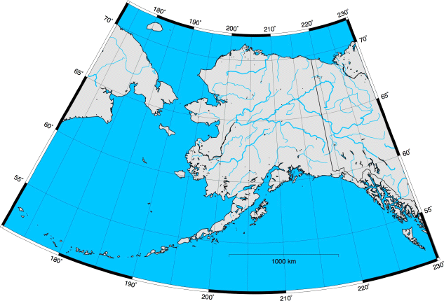
The Result
As seen below, we now have a nice map of Alaska, with grid lines, borders and degree annotations. The land and water is filled as we specified and the scale bar is sitting nicely in the Gulf of Alaska.
 February 22, 2008
·
February 22, 2008
·  admin ·
  No Comments
 Tags: gmt · Posted in: GMT


